Скачать или смотреть Excel Module 3 SAM Project A | Freedom Financial | CREATE A SALES REPORT

Excel Module 3 SAM Project A | Freedom Financial | CREATE A SALES REPORT #shellycashman

If you directly want to get the project from us then contact us on our Whatsapp. Link is given here,

Whatsapp Contact Link:
https://api.whatsapp.com/message/4B6NMKKBK...

Whatsapp Number:
+919116641093
+918005564456

Gmail Id:
[email protected]

We are providing help in all Online Courses, Computer Science, Business and Management, Business Math, Business and Finance, Business and Accounting, Human Resource Management, History, English.

PROJECT STEPS
1. Alexi Fisher is the director of recruiting and business development for Freedom Financial in San Diego, California. She has been analyzing sales and dividends for finance professionals in an Excel workbook and has asked you to help her complete the analysis.

Go to the Sales worksheet. Rename the Sales worksheet as Sales and Dividends, which is a more accurate name.
2. Unfreeze column A so it is not displayed when you scroll horizontally.
3. Middle align and center align the contents of the merged cell A1 to improve the appearance of the worksheet title.
4. In cell I3, insert a formula that uses the NOW function to display today's date.
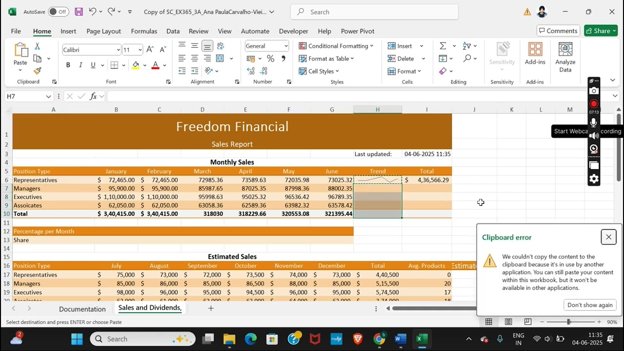
5. Fill the range C6:G10 with the formatting from the range B6:B10 to use a consistent number format for the sales data.
6. Alexi wants to show the sales trend for each position and month from January to June. Provide this information as follows:
a. In cell H6, insert a Line sparkline based on the data in the range B6:G6.
b. Use the Fill Handle to fill the range H7:H10 without formatting based on the contents of cell H6.
c. Change the color of the sparklines in the range H6:H10 to Olive Green, Text 2 (4th column, 1st row of the Theme Colors palette) to emphasize them.
d. Show a High Point and a Low Point in the sparklines to make those values easy to identify.
7. Copy the formula in cell I6 and paste it in the range I7:I10, pasting only the formula and number formatting, to include sales totals.
8. Alexi wants to determine how the sales of each month contributed to the total sales. Calculate this information for her as follows:
a. In cell B13, insert a formula without using a function that divides the total sales for January (cell B10) by the total sales to date (cell I10).
b. Use an absolute reference to cell I10 in the formula.
c. Use the Fill Handle to fill the range C13:G13 with the formula in cell B13.
9. Alexi would like to increase the average number of product sales per month, and specifically how many representative financial products she needs to reach the goal of 20 products per month.

Use Goal Seek to set the average number of product sales for all positions (cell I21) to the value of 20 by changing the average number of representative products (cell I17).
10. Format the text in cell J16 to clarify what it refers to as follows:
a. Merge and center the range J16:J21.
b. Rotate the text down to -90 degrees in the merged cell so that the text reads from top to bottom.
c. Change the width of column J to 7.00.
11. Alexi also needs to calculate the dividends earned each month. If the company earns $200,000 or more in a month, the dividend is 30% of the sales. If the company earns less than $200,000 in a month, the dividend is 25% of the sales. Calculate the dividends as follows:
a. In cell B25, enter a formula that uses the IF function and tests whether the total sales for January (cell B10) is greater than or equal to 200000.
b. If the condition is true, multiply the total sales for January (cell B10) by 0.30 to calculate a dividend of 30%.
c. If the condition is false, multiply the total sales for January (cell B10) by 0.25 to calculate a dividend of 25%.
d. Use the Fill Handle to fill the range C25:G25 with the formula in cell B25 to calculate the dividends for February through June.
12. Change the sparklines in the range H25:H26 as follows to use a more meaningful format:
a. Change the Column sparklines to Line sparklines.
b. Apply the sparkline style Dark Blue, Sparkline Style Dark #6 (6th column, 5th row of the Sparkline Styles palette) [Mac Hint: 2nd column, 5th row of the Sparkline Styles palette] to make the sparklines easier to see.
13. Delete row 35, which contains information Alexi does not need anymore.
Your workbook should look like the Final Figures on the following pages. Save your changes, close the workbook, and then exit Excel. Follow the directions on the website to submit your completed project.