Consumption function in Macroeconomics or The Keynesian Theory of Consumption. In this video will start to examine the market for goods and services. More precisely the consumption function also called Keynesian consumption function.
The level of GDP, the overall price level, and the level of employment—three chief concerns of macroeconomists—are influenced by events in three broadly defined “markets”: Goods-and-services market, Financial (money) market, Labor market
In any given period, there is an exact equality between aggregate output (production) and aggregate income. You should be reminded of this fact whenever you encounter the combined term aggregate output (income) (Y).
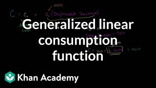
The consumption function, or Keynesian consumption function, is an economic formula that represents the functional relationship between total consumption and gross national income. It was introduced by British economist John Maynard Keynes, who argued the function could be used to track and predict total aggregate consumption expenditures.
A consumption function for an individual household shows the level of consumption at each level of household income.
Consumption function, in economics, the relationship between consumer spending and the various factors determining it. At the household or family level, these factors may include income, wealth, expectations about the level and riskiness of future income or wealth, interest rates, age, education, and family size. The consumption function is also influenced by the consumer’s preferences
With a straight line consumption curve, we can use the following equation to describe the curve: C = a + bY
The aggregate consumption function shows the level of aggregate consumption at each level of aggregate income.
The upward slope indicates that higher levels of income lead to higher levels of consumption spending.
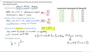
marginal propensity to consume (MPC) That fraction of a change in income that is consumed, or spent. Marginal propensity to consume ≡ slope of consumption function ≡ ∆𝐶/∆𝑌
marginal propensity to save (MPS) That fraction of a change in income that is saved. Marginal propensity to save ≡ slope of saving function ≡ ∆𝑆/∆𝑌
MPC + MPS ≡ 1
identity Something that is always true.
aggregate saving (S) The part of aggregate income that is not consumed.
Because S ≡ Y – C, it is easy to derive the saving function from the consumption function.
A 45° line drawn from the origin can be used as a convenient tool to compare consumption and income graphically.
At Y = 200, consumption is 250.
The 45° line shows us that consumption is larger than income by 50. the 45-degree line, which represents in this graph the set of points where aggregate consumption in the economy is equal to output, or national income.
Thus, S ≡ Y – C = -50.
At Y = 800, consumption is less than income by 100.
Thus, S = 100 when Y = 800.
In general, planned investment is the amount of investment firms plan to undertake during a year. Actual investment is the amount of investment actually undertaken during a year. If actual investment is greater than planned investment, then inventories go up, since inventories are part of capital. This increase in inventories may lead firms to reduce output.
For the time being, we will assume that planned investment is fixed.
It does not change when income changes, so its graph is a horizontal line.
Unlike consumption, Investment depends more on interest rates and on business expectations than on level of income.
Investment Function – The relationship between the amount businesses plan to invest and the level of income in the economy, other things constant.
The simplest investment function assumes that planned investment is autonomous investment is independent of level of income.
0:00 Introduction
1:19 Keynesian Consumption Function
2:25 Consumption Line Equation
3:13 MPC and MPS
5:40 Consumption numerical example
7:22 Saving Function
10:15 Planned investment
#Macroeconomics #Consumptionfunction#MPC
for more videos: / @socratghadban


Информация по комментариям в разработке