Скачать или смотреть Experiments 3D - Case study: a 4-factor system using computer software

Videos used in the Coursera course: Experimentation for Improvement. Join the course for FREE at https://www.coursera.org/learn/experi...

These videos are also part of the free online book, "Process Improvement using Data", http://yint.org/pid

Full script for the video: http://yint.org/scripts/3D
--------------------
Let's look at a good case study now, involving four factors, and two outcome variables. We're stepping up the complexity here a little bit. This is a good question, from the textbook by Box, Hunter and Hunter.

It's a case study where we we are using solar panels, with a storage tank. The outcome values were from a computer simulation.

Now just a quick piece of advice when using simulations. Running simulations is often really easy. But there's a temptation to really do this inefficiently. I often see people just playing around with the software, trying out different values, until they get an answer they like. You shouldn't treat simulations any differently from real life. Always use a systematic method.

In this case we're going to use a set of experiments as our systematic method. There are two key advantages though to using simulations. You can run the simulations in parallel at very little cost and secondly, you don't have to randomize the order of experiments. And the reason for that is quite simple.

When you repeat the simulation, you get the same answer, so the need for randomization isn't there anymore, which was, minimize the impact of disturbances. Be careful though: certain computer experiments, when repeated, don't give identical results. So then you should randomize. In fact, I always recommend you randomize. The cost of doing so if very minimal, and it guards against all sorts of problems. More on that in the next module though.

Let's go back to the solar panel system. There are four factors.
A: the total amount of insulation or sunlight received;
B: the capacity of the storage tank;
C: the water flow rate through the absorber; and
D: the intermittency of the sunlight.

You can read more about these types of systems, by following this link.

The two outcome variables were "y_1" the collection efficiency, and "y_2" the energy delivery efficiency.

You should be able to quickly tell how many experiments will be done, if each factor is operated at the low level and the high level.

You should have: two to the power of four (2\^4) which is 16. So 16 experiments were run, and I've put the results and the R code here on the screen. They're available on the course website. Copy and paste that code and follow along with me for the rest of the video.

So here we define the four factors: A, B, C and D, and I've manually typed in the two outcome variables, "y_1" and "y_2". This is what you would do in practice, but to make things a bit simpler, and to avoid typing errors, you can also use the PID package in R.

In a prior video I showed how you can download and install that package, to extend R's capability. That package includes the numeric results for this case study. And you can get that dataset by typing the following command: data(solar).

So since we ran 16 experiments, we are able to estimate 16 parameters: there are four main effects (one for A, B, C and D). There are 6 two-factor interactions, there are 4 three-factor interactions, and then the single four-factor interaction. That's a total of 15 parameters, and it adds to 16 if you count the intercept. The software can create all of this for you, very compactly with the "lm(...)" command, as shown here.

The reason why this A*B*C*D concept works is because of the principle of model hierarchy.

Let's take a simple example: if you wrote just A*B, then R will expand that to include factor A and factor B in the model. After all, you can't have the two factor interaction A*B if you don't also have factor A and factor B.

Similarly, when R encounters A*B*C, it ensures that the AB interaction is present, as well as factor C. But, we've already mentioned that the AB will be expanded into factors A and B. So it will ensure the BC interaction is present, and in a similar line of thinking, the AC interaction will also be present.

So now you can understand why when we write A*B*C*D here in the lm(...) command, R will recursively expand this into all the main effects, all the two factor interactions, all the 3 factor interactions as well as the 4 factor interaction. It is as if we had written it all out by hand as shown here. But obviously that is tedious, and error-prone, so let R do the work for you.

Now let's build those two separate linear models: for the collection efficiency, "y1", and for the energy delivery efficiency, "y2".

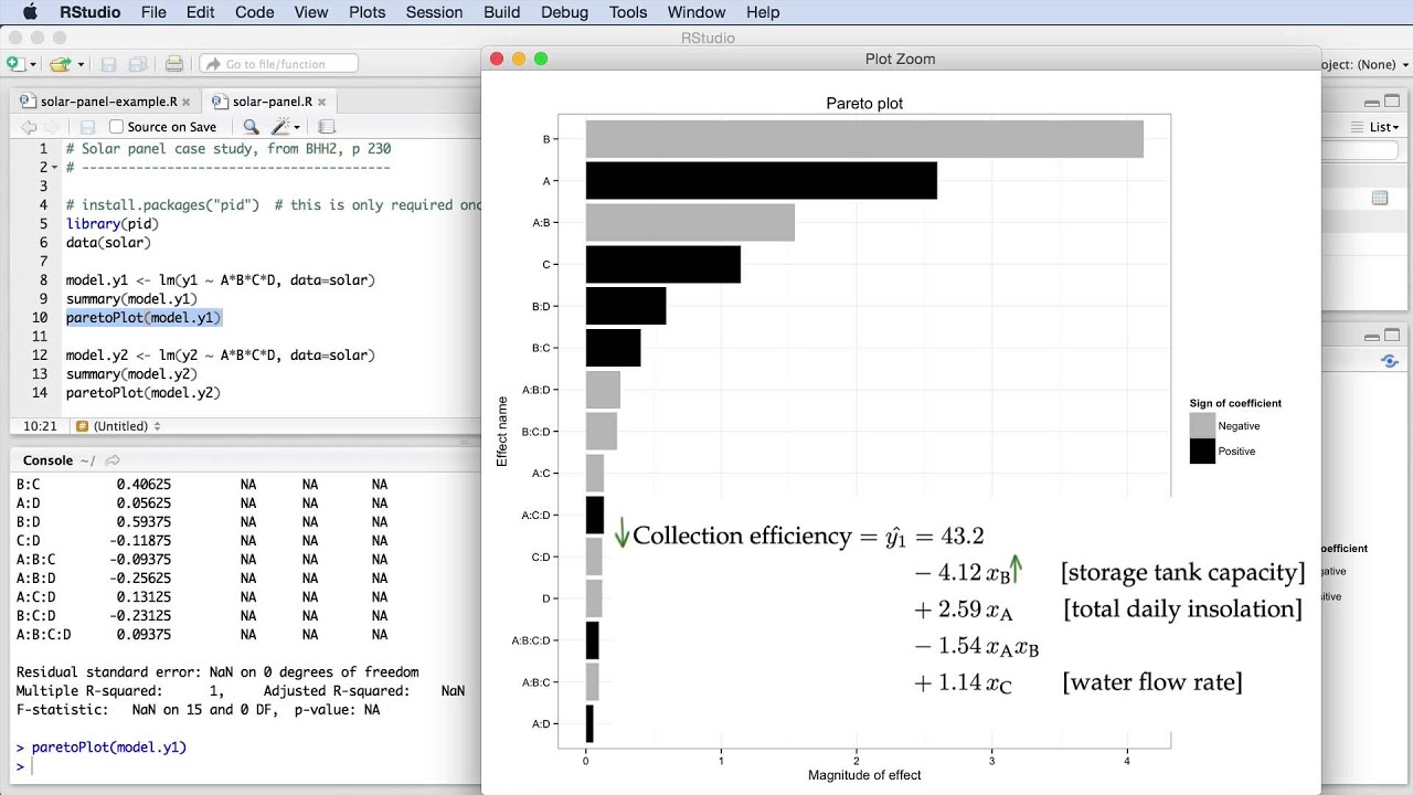
If you use the summary(...) command, as we've done before, it might be fairly difficult to quickly locate what the important factors are that influence y_1. Rather let's use the Pareto plot to show us what the important parameters are.

Here it is: the grey bars represent the terms ...