Скачать или смотреть Colliding spirals in the Rock-Paper-Scissors equation 4: phase and vorticity

This new episode of our series on colliding spirals in the Rock-Paper-Scissors reaction-diffusion equation with increasing viscosity shows two new visualizations, combining different information in the z-coordinate of the plot, and in the color hue:
Gradient of phase: 0:00
Vorticity and phase: 1:20
Both parts show quantities related to an angular variable, let us call it "phase", which roughly depends on the predominant chemical in the reaction. In the first part, the z-component shows the norm of the gradient of the phase, indicating how fast the phase changes in space. The hue depends on the direction of the gradient, as in the video    • Direction of rotation in the Rock-Paper-Sc...  
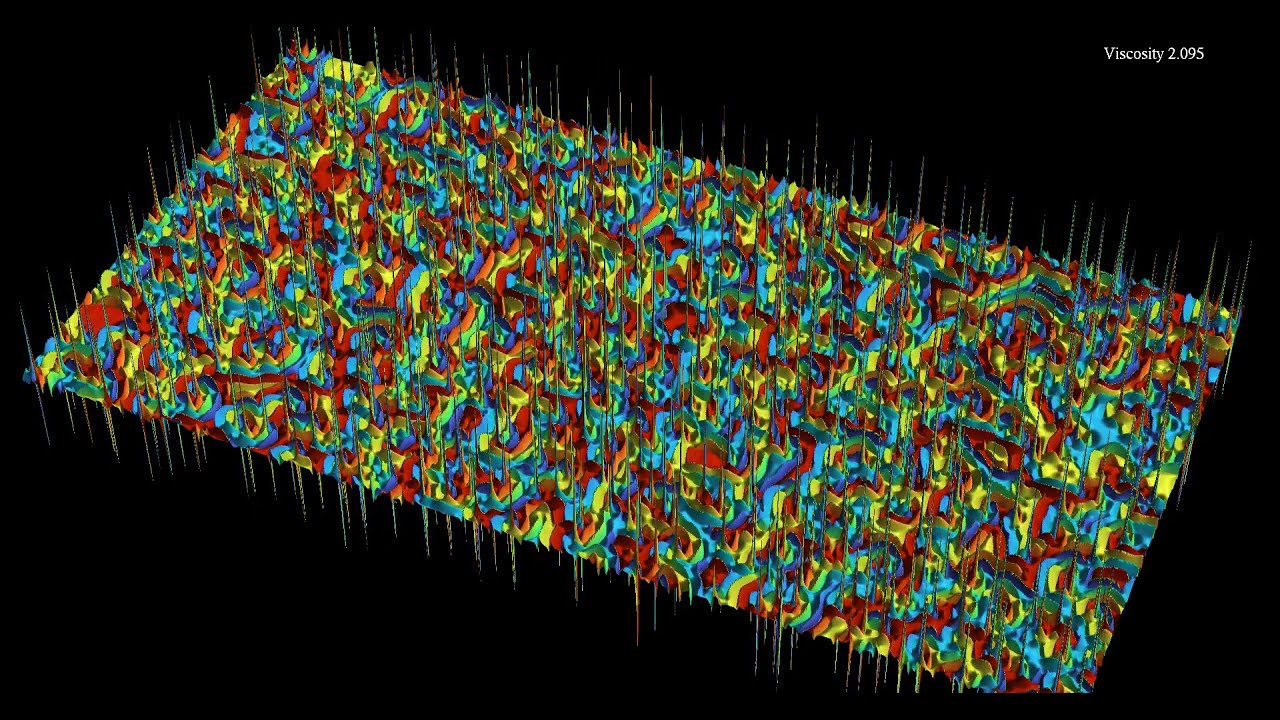
In the second part, the z coordinate shows the "vorticity" of the solution, see below for details. The vorticity diverges at the center of spirals, and allows to observe a few collisions of counter-rotating spirals, in which the spikes pairwise annihilate. The color hue indicates the phase itself, with red, yellow and blue representing locations where one of the three chemicals is predominant.
The reaction-diffusion equation is defined as follows. At each point in space and time, there are three concentrations u, v, and w of chemicals, that appear as red, blue and green in the video    • Larger spirals in the Rock-Paper-Scissors ...   . Denoting by rho = u + v + w the total concentration, the system of equations is given by
d_t u = D(t)*Delta(u) + u*(1 - rho - a*v)
d_t v = D(t)*Delta(v) + v*(1 - rho - a*w)
d_t w = D(t)*Delta(w) + w*(1 - rho - a*u)
where Delta denotes the Laplace operator, which performs a local average, and the parameter a is equal here to 0.75 while D(t) increases from 0.05 to 5 in the course of the simulation. The terms proportional to a*v, a*w and a*u denote reaction terms, in which Red is beaten by Blue, Blue is beaten be Green, and Green is beaten by Red. The situation is thus similar to the Rock-Paper-Scissors game (see https://en.wikipedia.org/wiki/Rock_pa... ), and there exist simpler cellular automata with similar properties, see for instance https://softologyblog.wordpress.com/2...
To obtain the vorticity, the values of u, v and w are first converted into an angle, or phase with the following steps:
divide u and v by the total density rho = u + v + w
set x = (u - 1/3) + (v - 1/3)/2 and y = (v - 1/3)*sqrt(3)/2
convert (x,y) to polar coordinates, the angular part defining the phase.
The resulting transformation from (u,v,w) to (x,y) is similar to a discrete Fourier transform with 3 modes.
The vorticity is then obtained by computing the curl (or rotational) of the gradient of the polar angle. For a smooth field, the curl of the gradient is zero. However, the curl has singularities where the gradient is not defined, as in the center of spirals. This allows to make the center of the spirals visible as peaks (I'm not sure where the other spirals come from, they may be due to round-off errors). In the course of the simulation, the viscosity parameter of the equation increases, making centers of vortices and anti-vortices (rotating in opposing directions) annihilate.

Render time: 1 hours 20 minutes
Color schemes: Part 1 - Twilight
Part 2 - Turbo, by Anton Mikhailov
https://gist.github.com/mikhailov-wor...

Music: "Space Trooper" by DivKid‪@DivKid‬

See also https://images.math.cnrs.fr/Des-ondes... for more explanations (in French) on a few previous simulations of wave equations.

The simulation solves a reaction-diffusion equation by discretization.
C code: https://github.com/nilsberglund-orlea...
https://www.idpoisson.fr/berglund/sof...