In this video we discuss how to calculate the standard deviation of a data set by hand in excel, by creating a formula. We go through this in detail step by step
Transcript/notes (partial)
Here in column B is a sample data set of the yards receiving for a receiver over a 17 game period. We are going to go through how to calculate standard deviation for this data set, in excel by hand.
Looking at the variables, we need to know x bar, or the mean or average of the data set, which we are going to put in column C. To calculate this, we left double click on cell C2, so it is highlighted. Next, we type in the letters su and a pop up box will appear, in the box we left double click on sum.
Now we left click and hold on cell B2, then drag down to the bottom of the data, cell B18, and then release the click and hold. Next we type in a closed parenthesis to close off the sum function. Next, we need to divide by the number of games, which is 17, so type in a division sign, which is a forward slash in excel. We can type in 17, but, if you have a lot of data points, it is easier to use the count function, which will count the number of cells.
So, type in cou, and in the pop up box, left double click on count. Now, we left click and hold on cell A2, then drag down to the bottom, cell A18, and release the click and hold. Then type in a closed parenthesis to close off the count function, and then we hit the enter key and we have our answer of 102.88 rounded off.
The next thing we need to know, to calculate the standard deviation from the formula is x minus x bar. So, we are going to put this in column D, as I have labeled on the worksheet. To calculate this, we need to subtract the mean from each of the data points. So, we left click on cell D2, then type in an equals sign. Next we left click on the first data point, 77 in cell B2, and then we type in a minus sign. From here we left click on the average or x bar, cell C2, and then we can hit the enter key and we have our answer of negative 25.88 rounded off.
To make this easier to fill in the rest of column D, we need to modify the formula in cell D2, so we left double click on cell D2. And go over between the C and the 2 and type in a dollar sign, then hit the enter key. This tells excel reference this cell. Next, we left click again on cell D2 and go down to the bottom right corner of the cell and you will see the cursor turn black, from here, left click and hold and drag down to the bottom of the data, cell D18, and then release the click and hold, and as you see, the column has been filled in for the rest of the data points.
Looking at the formula, the next thing we need to do is square x minus x bar, which I have labeled in column E. So, left click on cell E2, then type in an equals sign. Next, we left click on the first value, cell D2, then type in a to a power symbol, a carrot sign, which is shift 6 on the keyboard. Now we type in a 2, because we are squaring it, then hit the enter key and we have our answer of 669.89 rounded.
Next, we left click again on cell E2 and go down to the bottom right corner of the cell and you will see the cursor turn black, from here, left click and hold and drag down to the bottom of the data, cell E18, and then release the click and hold, and as you see, the column has been filled in for the rest of the data points.
The next thing we need to do is find the sum of squares, which is the sum of the values in column E. To do this, left click and hold on cell E2, then drag down over the cell below the last value cell E19, then release the click and hold. From here, we go to the summation symbol in the editing section near the top of the worksheet, as you see here, and left click on it. And we have our answer of 51,493.76 rounded.
Now following the formula, we can calculate the standard deviation. I am going to put the answer in cell A23, so I left click on A23. Next, type in an open parenthesis, then we left click on the sum we just calculated, cell E19. Now we need to type in a division sign, a forward slash, then another open parenthesis. From here, we need to input n, the number of data points and we are going to use the count function again, So, type in cou, and in the pop up box, left double click on count.
Now, we left click and hold on cell A2, then drag down to the bottom, cell A18, and release the click and hold. Then type in a closed parenthesis to close off the count function. Next we type in a minus sign followed by a 1, then we need to type in 2 closed parentheses.
Chapters/Timestamps
0:00 Formula for standard deviation
0:13 Example start
0:23 Calculate the mean
0:56 Calculate x minus xbar
1:32 Adjust the formula for x minus xbar
2:15 Calculate x minus xbar squared
3:02 Calculate the sum of x minus xbar squared
3:34 Formula in excel to calculate the standard deviation


Информация по комментариям в разработке