Скачать или смотреть Shelly Cashman Excel 365 | Module 5: End of Module Project 2 | Business Matters

Shelly Cashman Excel 365 | Module 5: End of Module Project 2 | Business Matters #shellycashman

If you directly want to get the project from us then contact us on our Whatsapp. Link is given here,

Whatsapp Contact Link:
https://api.whatsapp.com/message/4B6N...

Whatsapp Number:
+919116641093
+918005564456

Gmail Id:
[email protected]

We are providing help in all Online Courses, Computer Science, Business and Management, Business Math, Business and Finance, Business and Accounting, Human Resource Management, History, English.


PROJECT STEPS
1. Ming Pei is the subscription manager for Business Matters, an online media company in New York City that provides news to subscribers about business and financial markets. She is tracking subscription information in an Excel workbook and asks for your help in analyzing the data. She also needs to complete a schedule for launching an online newsletter.

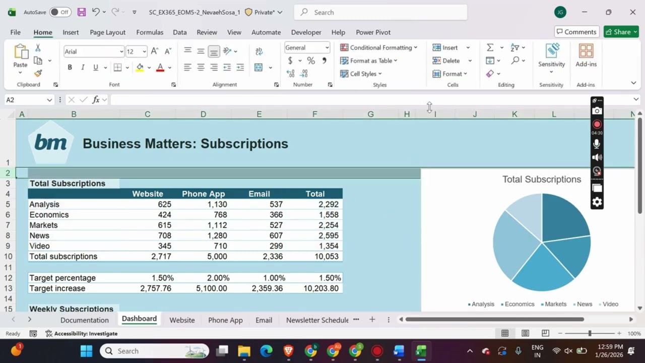
Go to the Dashboard worksheet. In the range C5:C9, Ming asks you to consolidate data that summarizes subscriptions made through the Business Matters website. In cell C5, insert a formula that references cell C17 on the Website worksheet to insert the total number of Analysis subscriptions made through the website during the last 12 weeks. Insert similar formulas in the range C6:C9 to include the totals for Economics, Markets, News, and Video subscriptions during the last 12 weeks.
2. The Total Subscriptions pie chart in the range I4:L11 compares the totals of each subscription source. Resize the chart to a height of 3" and a width of 5" to clarify the data. Position the chart so that the upper-left corner is in cell I2.
3. Add data labels to the chart on the outside end to make the chart easier to interpret, show only the category name and percentage values in the data labels, and then change the number format to Percentage with one decimal place. Remove the legend, which is now unnecessary.
4. Ming calculated the targeted number of subscriptions she wants to achieve for the rest of the year, but wants you to round the increase amount to simplify the values. Add the ROUND function to the formulas in the range C13:F13 to round the results to 0 decimal places, and then decrease the number of decimal places shown to none.
5. In the range B16:G29, Ming wants you to summarize the weekly subscription data for all three sources of subscriptions.
In cell C17, enter a formula using the SUM function and a 3-D reference to total the number of Analysis subscriptions in Week 1 (cell C5) from the Website, Phone App, and Email worksheets. Fill the range C18:C28 with the formula in cell C17 to consolidate the Analysis subscription data for the remaining weeks. Fill the range D17:G28 with the formulas in the range C15:C26 to consolidate the data for Economics, Markets, News, and Video subscriptions.
6. Go to the Website worksheet. Use the text in the range B5:B6 to fill the range B7:B16 with the week numbers.
7. Ming has set a goal of 320 weekly subscriptions from the Business Matters website by week 24. She asks you to identify the number of subscriptions needed every four weeks to meet this goal. In the range C21:F21, project the subscriptions per week by filling the series with a linear trend. She also asks you to project an increase in subscriptions by 5 percent every four weeks. In the range C23:F23, project the subscriptions based on a growth series using 1.05 as the step value.
8. Go to the Newsletter Schedule worksheet, which contains the beginnings of a schedule for publishing an online newsletter. In cell C3, enter a formula using the DATE function to enter September 9, 2029 as the date.
9. For milestones 2–10, the dates are five days after the previous start date. To exclude weekends for those days, enter a formula in cell D7 using the WORKDAY function that adds 5 days to the date in cell D6. Fill the range D8:D15 with the formula in cell D7 to complete the schedule.
10. Ming asks you to remove the year from the display of the newsletter schedule so the dates are easier to read. Add a custom format to the range D5:E15 that shows only the month (m), a slash (/), and the day (d), as in 9/12.
11. Move the Newsletter Timeline chart to the Dashboard worksheet. Position the chart so its upper-left corner is in cell I16 and its lower-right corner is in cell N29 without resizing the chart.
12. Change the number format of the horizontal axis values in the Newsletter Timeline chart to display dates with a three-character month name, a space, and the day, as in Sep 9.
Your workbook should look like the Final Figures on the following pages. Save your changes, close the workbook, and then exit Excel. Follow the directions on the website to submit your completed project.